本质上是一个准备NLP面试的笔记，所以只谈谈BERT和LDA。

BERT的全称为Bidirectional Encoder Representation from Transformers，是一个预训练的语言表征模型。它强调了不再像以往一样采用传统的单向语言模型或者把两个单向语言模型进行浅层拼接的方法进行预训练，而是采用新的masked language model（MLM），以致能生成深度的双向语言表征。

1）采用MLM对双向的Transformers进行预训练，以生成深层的双向语言表征。

2）预训练后，只需要添加一个额外的输出层进行fine-tune，就可以在各种各样的下游任务中取得state-of-the-art的表现。在这过程中并不需要对BERT进行任务特定的结构修改。

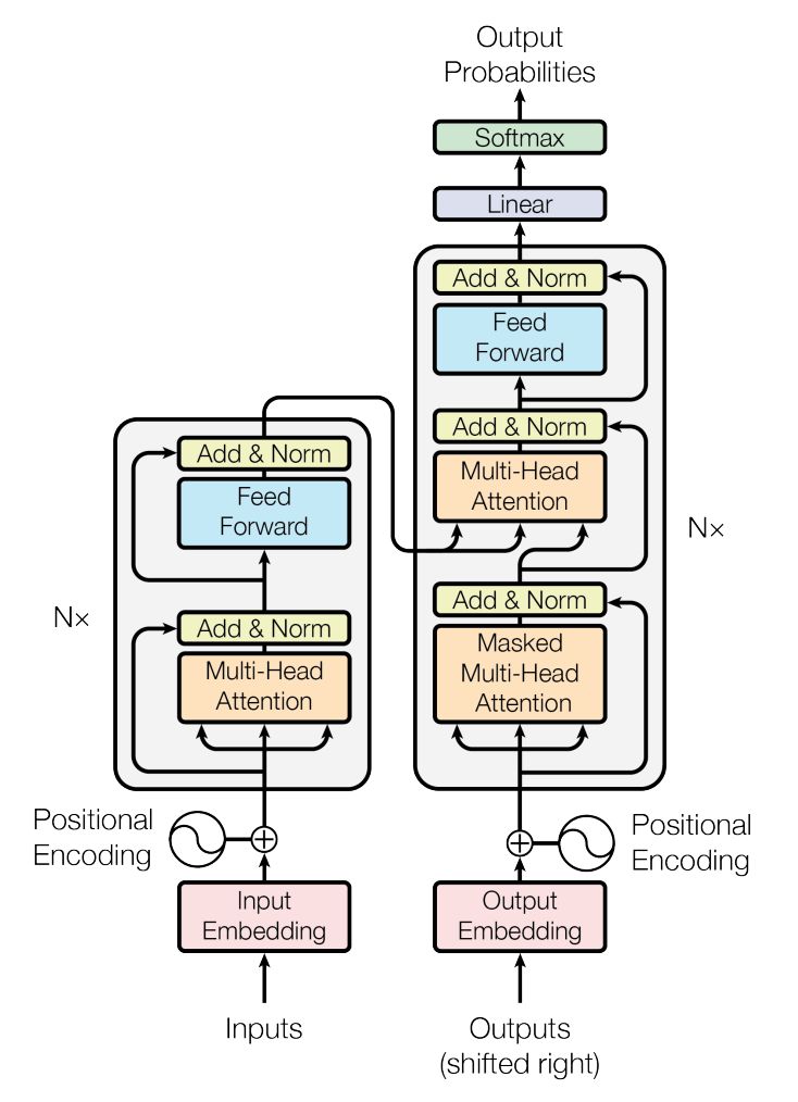
Transformer

Transformer 在2017年 Attention is All You Need 中提出，提出的一种模型架构，这篇论文里只针对机器翻译这一种场景做了实验，完爆当时的SOTA，并且由于Encoder端是并行计算的，训练的时间被大大缩短了。

Multi-head Attention其实就是多个Self-Attention结构的结合，每个head学习到在不同表示空间中的特征，两个head学习到的Attention侧重点可能略有不同，这样给了模型更大的容量。

它开创性的思想，颠覆了以往序列建模和RNN划等号的思路，现在被广泛应用于NLP的各个领域。目前在NLP各业务全面开花的语言模型如GPT, BERT等，都是基于Transformer模型。

机器翻译是从RNN开始跨入神经网络时代的，大致经历了Simple RNN, Contextualize RNN, Contextualized RNN with attention, Transformer(2017)几个阶段。

• Simple RNN

An Encoder-Decoder structure. Encoder

Contextualized RNN：为了解决上述第二个问题，即encoder output随着decoder timestep增加而信息衰减的问题，有人提出了一种加了context的RNN sequence to sequence模型：decoder在每个timestep的input上都会加上一个context。为了方便理解，我们可以把这看作是encoded source sentence。这样就可以在decoder的每一步，都把源端的整个句子的信息和target端当前的token一起输入到RNN中，防止源端的context信息随着timestep的增长而衰减。

context对于每个timestep都是静态的(encoder端的final hidden states，或者是所有timestep的output的平均值)。但是每个decoder端的token在解码时用到的context真的应该是一样的吗？

Contextualized RNN with soft align (Attention)

在每个timestep输入到decoder RNN结构中之前，会用当前的输入token的vector与encoder output中的每一个position的vector作一个”attention”操作，这个”attention”操作的目的就是计算当前token与每个position之间的”相关度”，从而决定每个position的vector在最终该timestep的context中占的比重有多少。最终的context即encoder output每个位置vector表达的加权平均。

Self Attention

首先，关于 Attention 机制：

将注意力放到某些事物上，而忽略另一些，这就是注意力机制（Attention Mechanism）。

在深度学习领域，模型往往需要接收和处理大量的数据，然而在特定的某个时刻，往往只有少部分的某些数据是重要的，Attention 机制就适用于这种情况。

假定输入为 Q(Query), Memory 中以键值对 (K,V) 的形式存储上下文。那么注意力机制其实是 Query 到一系列键值对 (Key, Value) 上的映射函数。

self-attention的q, k, v都是同一个输入, 即当前序列由上一层输出的高维表达。

BERT

BERT Details from the Original Paper

翻译一下 BERT 的原文第三节，细节与实现部分。

We introduce BERT and its detailed implementation in this section. There are two steps in our framework: pre-training and fine-tuning. During pre-training, the model is trained on unlabeled data over different pre-training tasks. For finetuning, the BERT model is first initialized with the pre-trained parameters, and all of the parameters are fine-tuned using labeled data from the downstream tasks. Each downstream task has separate fine-tuned models, even though they are initialized with the same pre-trained parameters.

The question-answering example in Figure 1 will serve as a running example for this section.

我们在这部分介绍 BERT 和它的细节实现。我们的框架包含两部分，pre-training and fine-tuning。Pre-training 时模型通过不同pre-training 任务在无标签数据(unlabeled data)上训练。关于 finetuning，BERT 模型首先用 pre-trained 的参数初始化，然后所有参数用下游任务的标签数据(labeled data) fine-tune。每个下游任务有独自的 fine-tuned 过的模型，尽管他们都用一样的 pre-trained 参数初始化。

总之图1是本节例子。

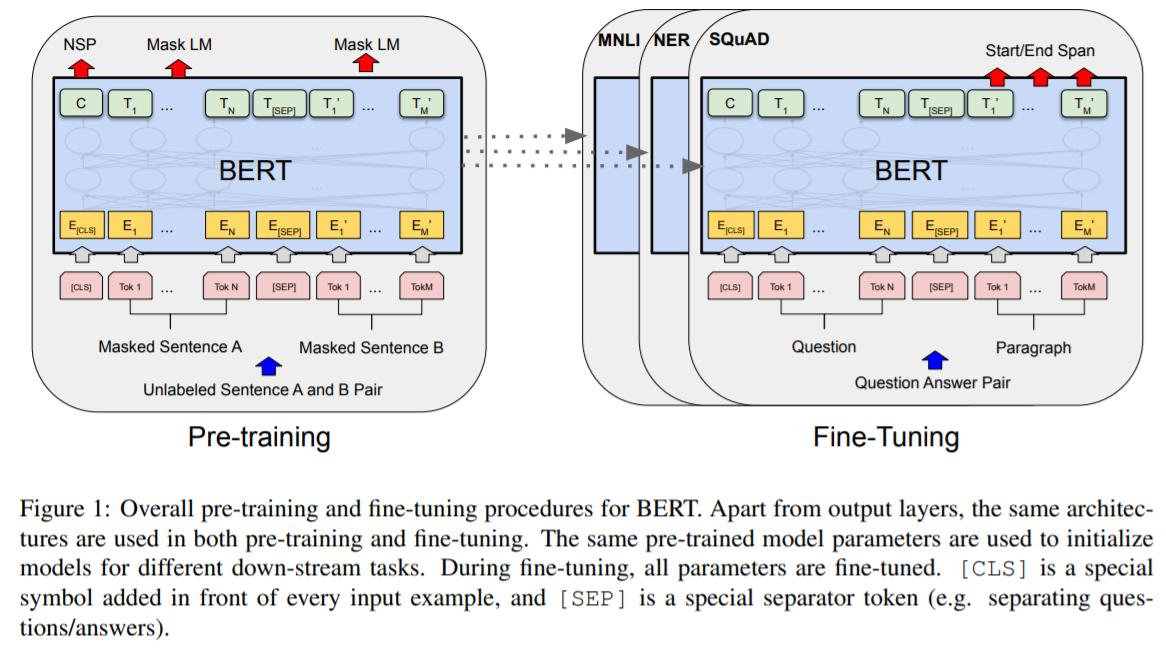
A distinctive feature of BERT is its unified architecture across different tasks. There is minimal difference between the pre-trained architecture and the final downstream architecture.

BERT 的一个独有特征是它跨不同任务间的统一结构。

Model Architecture BERT’s model architecture is a multi-layer bidirectional Transformer encoder based on the original implementation described in Vaswani et al. (2017) and released in the tensor2tensor library. 1 Because the use of Transformers has become common and our implementation is almost identical to the original, we will omit an exhaustive background description of the model architecture and refer readers to Vaswani et al. (2017) as well as excellent guides such as “The Annotated Transformer.” 2

1 > https://github.com/tensorflow/tensor2tensor

2 > http://nlp.seas.harvard.edu/2018/04/03/attention.html

模型结构 BERT 的模型结构是一种多层双向 Transformer 编码器，基于 Vaswani 等人的原版实现。总之是用的很多，实现得又一样，我们就不谈了嗷。去参考人的论文或者 The Annotated Transformer 就完事儿了。

In this work, we denote the number of layers (i.e., Transformer blocks) as L, the hidden size as H, and the number of self-attention heads as A. 3 We primarily report results on two model sizes:

BERTBASE (L=12, H=768, A=12, Total Parameters=110M)

and

BERTLARGE (L=24, H=1024, A=16, Total Parameters=340M).

BERTBASE was chosen to have the same model size as OpenAI GPT for comparison purposes. Critically, however, the BERT Transformer uses bidirectional self-attention, while the GPT Transformer uses constrained self-attention where every token can only attend to context to its left. 4

3 > In all cases we set the feed-forward/filter size to be 4H, i.e., 3072 for the H = 768 and 4096 for the H = 1024.

4 > We note that in the literature the bidirectional Transformer is often referred to as a “Transformer encoder” while the left-context-only version is referred to as a “Transformer decoder” since it can be used for text generation.

在这项工作中，我们记网络层数(即Transformer blocks)为 L，隐藏层大小为 H，自关注头(self-attention heads)数量为 A。我们主要报告两周模型大小的结果：BERTBASE 和 BERTLARGE。为比较，BERTBASE 被选择为和 OpenAI GPT 有相同模型尺寸。然而重要的是，BERT Transformer 使用双向(bidirectional) self-attention，而 GPT Transformer 使用受限的 self-attention，其中每个词(token)只能照顾到左侧的上下文。

Input/Output Representations To make BERT handle a variety of down-stream tasks, our input representation is able to unambiguously represent both a single sentence and a pair of sentences (e.g., <Question, Answer>) in one token sequence. Throughout this work, a “sentence” can be an arbitrary span of contiguous text, rather than an actual linguistic sentence. A “sequence” refers to the input token sequence to BERT, which may be a single sentence or two sentences packed together.

输入/输出表示

为使 BERT 处理多样的下游任务，我们的输入表示能在一个 token 序列中明确表示一个单独句子和一对句子（比如<Question, Answer>）。本工作中，“句子”可以是任意区间连续文本，而非实际意义上的语言学文本。一个“句子”指BERT 的输入 token 序列，可能是一个单独句子或者是两个打包在一起的句子。

We use WordPiece embeddings (Wu et al., 2016) with a 30,000 token vocabulary. The first token of every sequence is always a special classification token ([CLS]). The final hidden state corresponding to this token is used as the aggregate sequence representation for classification tasks. Sentence pairs are packed together into a single sequence. We differentiate the sentences in two ways. First, we separate them with a special token ([SEP]). Second, we add a learned embedding to every token indicating whether it belongs to sentence A or sentence B. As shown in Figure 1, we denote input embedding as E, the final hidden vector of the special [CLS] token as C ∈ R^H, and the final hidden vector for the i-th input token as T_i ∈ R^H.

我们使用有 30,000 个 token 词汇的 WordPiece embedding(Wu 等人的)。每个序列的第一个 token 永远是一个特殊的分类 token ([CLS])。对应这个 token 的最后的隐藏状态用来做分类任务的集合序列表示(aggregate sequence representation)。句子对被分装在一起形成一个单独的序列。我们用两种方法区分开句子。一种是，我们用特殊 token ([SEP]) 划分句子。还有一种是我们给每个 token 加一个学习好的(learned) embedding 来表示它属于句子 A 或者 B。如图 1 所示，我们记输入 embedding 为 E，特殊 token [CLS] 的最终隐藏向量为 C ∈ R^H， 第 i 个输入 token 的最终隐藏向量为 T_i ∈ R^H。

For a given token, its input representation is constructed by summing the corresponding token, segment, and position embeddings. A visualization of this construction can be seen in Figure 2.

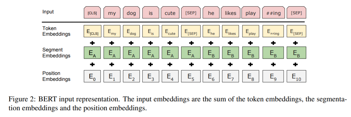
对于给出的 token，他的输入表示由对应的词符、分段、位置embedding(token embedding, segment embedding, and position embedding) 加和构成。图 2 可以看到这种构成的可视化。

3.1 Pre-training BERT

Unlike Peters et al. (2018a) and Radford et al. (2018), we do not use traditional left-to-right or right-to-left language models to pre-train BERT. Instead, we pre-train BERT using two unsupervised tasks, described in this section. This step is presented in the left part of Figure 1.

不像别人，我们不用传统从左到右或者从右到左的语言模型来预训练 BERT。我们用两个无监督任务来预训练 BERT，在本节介绍。这一步展现在图 1 的左侧。

Task #1: Masked LM Intuitively, it is reasonable to believe that a deep bidirectional model is strictly more powerful than either a left-to-right model or the shallow concatenation of a left-to-right and a right-to-left model. Unfortunately, standard conditional language models can only be trained left-to-right or right-to-left, since bidirectional conditioning would allow each word to indirectly “see itself”, and the model could trivially predict the target word in a multi-layered context.

任务 #1: 屏蔽语言模型 直觉上有理由相信一个深度双向模型比一个从左到右的模型或者浅层连接的从左到右和从右到左模型严格说来更强大。不幸的是，标准条件语言模型只能被从左到右或者从右到左地训练，因为双向条件将允许每个词间接地“看到自己”，从而模型可以在多层上下文中非常容易地预测目标词。

In order to train a deep bidirectional representation, we simply mask some percentage of the input tokens at random, and then predict those masked tokens. We refer to this procedure as a “masked LM” (MLM), although it is often referred to as a Cloze task in the literature (Taylor, 1953). In this case, the final hidden vectors corresponding to the mask tokens are fed into an output softmax over the vocabulary, as in a standard LM. In all of our experiments, we mask 15% of all WordPiece tokens in each sequence at random. In contrast to denoising auto-encoders (Vincent et al., 2008), we only predict the masked words rather than reconstructing the entire input.

为训练一个深度双向表示，我们简单地随机屏蔽(mask)一部分输入 token，然后预测那些被屏蔽的 token。这个步骤我愿称之为“屏蔽语言模型(masked LM)”(MLM)，虽然这常在文学上被称为完形填空。在这种情况下，对应被屏蔽的 token 的最终隐藏向量被喂进词汇表上的输出 softmax 里，就像在标准 LM 模型里一样。在我们的所有实验中，我们在每个序列中随机屏蔽了 15% 的 WordPiece tokens。为了和去噪自编码器对比，我们只预测了屏蔽的词而非重建整个输入。

Although this allows us to obtain a bidirectional pre-trained model, a downside is that we are creating a mismatch between pre-training and fine-tuning, since the [MASK] token does not appear during fine-tuning. To mitigate this, we do not always replace “masked” words with the actual [MASK] token. The training data generator chooses 15% of the token positions at random for prediction. If the i-th token is chosen, we replace the i-th token with (1) the [MASK] token 80% of the time (2) a random token 10% of the time (3) the unchanged i-th token 10% of the time. Then, Ti will be used to predict the original token with cross entropy loss. We compare variations of this procedure in Appendix C.2.

尽管这允许我们获得一个双向预训练模型，一个缺陷是我们在制造一种 pre-training 和 fine-tuning 之间的不匹配，因为 [MASK] token 不会在 fine-tuning 的时候出现。为了解决这个，我们不总是用真正的 [MASK] token 替换被屏蔽的词。训练数据生成器随机选择 15% 的token 位置来预测。如果第 i 个 token 被选择，我们替换第 i 个 token 为：

(1) 80% 的时候，[MASK] token

(2) 10% 的时候，一个随机 token。

(3) 10% 的时候，第 i 个 token 不变。然后 T_i 会通过交叉熵损失被用于预测原始 token。

我们在附录 C.2 中比较了此过程的各种变体。

Task #2: Next Sentence Prediction (NSP) Many important downstream tasks such as Question Answering (QA) and Natural Language Inference (NLI) are based on understanding the relationship between two sentences, which is not directly captured by language modeling. In order to train a model that understands sentence relationships, we pre-train for a binarized next sentence prediction task that can be trivially generated from any monolingual corpus. Specifically, when choosing the sentences A and B for each pre-training example, 50% of the time B is the actual next sentence that follows A (labeled as IsNext), and 50% of the time it is a random sentence from the corpus (labeled as NotNext). As we show in Figure 1, C is used for next sentence prediction (NSP). 5 Despite its simplicity, we demonstrate in Section 5.1 that pre-training towards this task is very beneficial to both QA and NLI. 6

5 > The final model achieves 97%-98% accuracy on NSP.

6 > The vector C is not a meaningful sentence representation without fine-tuning, since it was trained with NSP.

The NSP task is closely related to representation learning objectives used in Jernite et al. (2017) and Logeswaran and Lee (2018). However, in prior work, only sentence embeddings are transferred to down-stream tasks, where BERT transfers all parameters to initialize end-task model parameters.

任务 #2: 下句预测(NSP) 许多重要下游任务比如 Question Answering (QA) 和 Natural Language Inference (NLI) 都基于理解两句子之间的关系，这不算能直接被语言模型捕捉的。为训练一个能理解句子关系的语言模型，我们预训练一个能被任何单语言语料简单生成的二值(binarized)下句预测任务。具体地说，当为每个预训练样本选择句子 A 和 B 时，50% 的时候 B 确实是接着 A 的下一个句子(标记为 IsNext)，还有 50% 的时候是语料中的随机句子(标记为 NotNext)。如我们在图 1 中知道的那样，C 被用于下句预测(NSP)。尽管它简单，我们在 5.1 节中展示对此任务的预训练对 QA 和 NLI 都非常有用。

NSP 任务与表示学习目标(representation learning objectives)很接近。然而在之前的工作中，只有句子的 embedding 被传输到下游任务中，而 BERT 传了所有参数去初始化末端任务模型的参数。

Pre-training data The pre-training procedure largely follows the existing literature on language model pre-training. For the pre-training corpus we use the BooksCorpus (800M words) (Zhu et al., 2015) and English Wikipedia (2,500M words). For Wikipedia we extract only the text passages and ignore lists, tables, and headers. It is critical to use a document-level corpus rather than a shuffled sentence-level corpus such as the Billion Word Benchmark (Chelba et al., 2013) in order to extract long contiguous sequences.

预训练数据 预训练过程大量跟随了已经存在语言模型预训练的文献。我们使用的预训练语料 BooksCorpus (800M 词) 和英文Wikipedia (2,500M 词)。对 Wikipedia 我们只提取文字段落并忽略列表、表格和标题。为了提取连续长序列，使用文档级别的语料而非混合的句子级别语料比如 Billion Word Benchmark 就非常重要。

3.2 Fine-tuning BERT

Fine-tuning is straightforward since the self-attention mechanism in the Transformer allows BERT to model many downstream tasks— whether they involve single text or text pairs—by swapping out the appropriate inputs and outputs. For applications involving text pairs, a common pattern is to independently encode text pairs before applying bidirectional cross attention, such as Parikh et al. (2016); Seo et al. (2017). BERT instead uses the self-attention mechanism to unify these two stages, as encoding a concatenated text pair with self-attention effectively includes bidirectional cross attention between two sentences.

Fine-tuning 很直接，因为 Transformer 里的 self-attention 机制允许 BERT 通过替换合适的输入和输出建模许多下游任务——无论他们包含单独文本还是文本对。对包含文本对的应用，一个寻常的模式是在应用双向交叉注意之前对文本对独立编码，比如 Parikh 等人. (2016); Seo 等人. (2017)做的。而 BERT 用 self-attention 机制来统一这两个阶段，因为用 self-attention 编码一个连接的文本对，实际上包括两个句子之间的双向交叉 attention。

For each task, we simply plug in the task specific inputs and outputs into BERT and finetune all the parameters end-to-end. At the input, sentence A and sentence B from pre-training are analogous to

(1) sentence pairs in paraphrasing,

(2) hypothesis-premise pairs in entailment,

(3) question-passage pairs in question answering, and

(4) a degenerate text-∅ pair in text classification or sequence tagging.

对每个任务，我们简单送入 BERT 特定于任务的输入和输出，然后端到端地 finetune 所有参数。在输入中，来自预训练的句子 A 和句子 B 相似于：

(1) 释义(paraphrasing) 中的句子对

(2) 蕴含(entailment) 中的假设-前提(hypothesis-premise)对

(3) question answering 中的问题-段落(question-passage)对

(4) 文本分类或序列标记 中的退化 text-∅ 对

At the output, the token representations are fed into an output layer for token-level tasks, such as sequence tagging or question answering, and the [CLS] representation is fed into an output layer for classification, such as entailment or sentiment analysis.

在输出中，token 表示被喂入一个输出层进行 token 级任务，比如 sequence tagging 或者 question answering，并且 [CLS] 表示被喂入一个输出层用于分类，比如 entailment 或者 sentiment analysis。

Compared to pre-training, fine-tuning is relatively inexpensive. All of the results in the paper can be replicated in at most 1 hour on a single Cloud TPU, or a few hours on a GPU, starting from the exact same pre-trained model.7 We describe the task-specific details in the corresponding subsections of Section 4. More details can be found in Appendix A.5.

和 pre-training 相比， fine-tuning 相对开销较小。所有文章的结果可以在单个的 Cloud TPU 上在一小时内复现，或在一个 GPU上用几个小时，从完全相同的预训练模型出发。

OpenAI GPT(Generative pre-trained transformer)，BERT是双向的Transformer block连接；就像单向rnn和双向rnn的区别，直觉上来讲效果会好一些。

对比ELMo，虽然都是“双向”，但目标函数其实是不同的。ELMo是分别以[公式] 和 [公式] 作为目标函数，独立训练处两个representation然后拼接，而BERT则是以 [公式] 作为目标函数训练LM。

分类：对于sequence-level的分类任务，BERT直接取第一个[CLS]token的最后一个隐含层状态 [公式] ，加一层权重 [公式] 后softmax预测标签概率 其他预测任务需要进行一些调整，可以调整的参数和取值范围有： Batch size: 16, 32 学习率 (Adam): 5e-5, 3e-5, 2e-5 epochs数量: 3, 4

到目前为止，所有提出的 BERT 结果都使用微调方法，即在预训练模型中添加一个简单的分类层，在下游任务上对所有参数进行共同微调。 但是，基于特征的方法，即从预训练的模型中提取固定的特征，也有一定的优势。 首先，并非所有任务都可以由 Transformer 编码器结构轻松表示，因此需要添加特定于任务的模型结构。 其次，预计算一次训练数据的昂贵表示，然后在这个表示之上用更便宜的模型运行许多实验，有很大的计算优势。

Latent Dirichlet Allocation

隐含狄利克雷分布，一种主题模型，它可以将【文档集】中每篇文档的主题以概率分布的形式给出，从而通过分析一些文档抽取出它们的主题（分布）出来后，便可以根据主题（分布）进行主题聚类或文本分类。同时，它是一种典型的词袋模型，即一篇文档是由一组词构成，词与词之间没有先后顺序的关系。此外，一篇文档可以包含多个主题，文档中每一个词都由其中的一个主题生成。

给pLSA加上贝叶斯框架，便是LDA

Probabilistic Latent Semantic Analysis

文档如何生成？pLSA中生成文档的整个过程便是选定文档生成主题，确定主题生成词。

先以一定的概率选取主题，再以一定的概率选取词。各个主题z在文档d中出现的概率分布称之为主题分布，且是一个多项分布。各个词语w在主题z下出现的概率分布称之为词分布，这个词分布也是一个多项分布。重复扔“文档-主题”骰子和”主题-词项“骰子，重复N次（产生N个词），完成一篇文档，重复这产生一篇文档的方法M次，则完成M篇文档。

——即是PLSA的文档生成模型，该模型假设一组共现(co-occurrence)词项关联着一个隐含的主题类别。

反过来，既然文档已经产生，那么如何 根据已经产生好的文档反推其主题呢？这个利用看到的文档推断其隐藏的主题（分布）的过程（其实也就是产生文档的逆过程），便是主题建模的目的：自动地发现文档集中的主题（分布）。

文档d和单词w自然是可被观察到的，但主题z却是隐藏的。 文档d和词w是我们得到的样本（ 样本随机，参数虽未知但固定，所以pLSA属于频率派思想。区别于下文要介绍的LDA中：样本固定，参数未知但不固定，是个随机变量，服从一定的分布，所以LDA属于贝叶斯派思想）可观测得到，所以对于任意一篇文档，其P(w_j|d_i) 是已知的。 从而可以根据大量已知的文档-词项信息，训练出文档-主题P(z_k|d_i) 和主题-词项P(w_j|z_k)。 故得到文档中每个词的生成概率为:

含待估计的两个未知变量。

待估计的参数中含有隐变量z，所以我们可以考虑EM算法(Expectation-maximization algorithm，期望最大算法)

综上，在pLSA中：

由于和未知，所以我们用EM算法去估计这个参数的值。 而后，用表示词项出现在主题中的概率，即，用表示主题出现在文档中的概率，即，从而把转换成了“主题-词项”矩阵Φ（主题生成词），把转换成了“文档-主题”矩阵Θ（文档生成主题）。 最终求解出、。

按照概率选择一篇文档 选定文档后，确定文章的主题分布 从主题分布中按照概率选择一个隐含的主题类别 选定后，确定主题下的词分布 从词分布中按照概率选择一个词 ”

下面，咱们对比下本文开头所述的LDA模型中一篇文档生成的方式是怎样的：

按照先验概率选择一篇文档 从狄利克雷分布（即Dirichlet分布）中取样生成文档 的主题分布，换言之，主题分布由超参数为的Dirichlet分布生成 从主题的多项式分布中取样生成文档第 j 个词的主题 从狄利克雷分布（即Dirichlet分布）中取样生成主题对应的词语分布，换言之，词语分布由参数为的Dirichlet分布生成 从词语的多项式分布中采样最终生成词语 ”

从上面两个过程可以看出，LDA在PLSA的基础上，为主题分布和词分布分别加了两个Dirichlet先验。

PLSA中，主题分布和词分布是唯一确定的，能明确的指出主题分布可能就是{教育：0.5，经济：0.3，交通：0.2}，词分布可能就是{大学：0.5，老师：0.3，课程：0.2}。 但在LDA中，主题分布和词分布不再唯一确定不变，即无法确切给出。例如主题分布可能是{教育：0.5，经济：0.3，交通：0.2}，也可能是{教育：0.6，经济：0.2，交通：0.2}，到底是哪个我们不再确定（即不知道），因为它是随机的可变化的。但再怎么变化，也依然服从一定的分布，即主题分布跟词分布由Dirichlet先验随机确定。

贝叶斯框架下的LDA中，我们不再认为主题分布（各个主题在文档中出现的概率分布）和词分布（各个词语在某个主题下出现的概率分布）是唯一确定的（而是随机变量），而是有很多种可能。但一篇文档总得对应一个主题分布和一个词分布吧，怎么办呢？LDA为它们弄了两个Dirichlet先验参数，这个Dirichlet先验为某篇文档随机抽取出某个主题分布和词分布。